How Does Instana Optimize Complex Queries in Process Time?
Instana aims to provide accurate and instantaneous app monitoring metrics in dashboards and unbounded analytics. These metrics are calculated based on millions of calls collected from systems under observation. Requests are stored in Clickhouse, a columnar database, and each request has hundreds of tags.
We use a variety of techniques to speed up the querying of this data. The most important of these is the use of materialized views (MV). The purpose here is to select the most frequently used tags such as service.name, endpoint.name, http.status and to pre-collect the metrics on these tags into groups of different sizes. The MV contains much less data than the original table, so it’s much faster to read, filter and aggregate from the view.
However, this approach has a limitation. There are 2 types of tags that cannot be included in the MV. Therefore, queries that filter or group by these tags cannot be optimized:
1. Tag with very high cardinality
Including tags like http.url in the MV will increase the number of lines in the MV. For example, if we add only endpoint.name in MV, endpoint /api/users/{id} will have only 1 line per minute if group size is 1 minute. However, if we add http.path additionally and the endpoint receives requests with hundreds of different paths like /api/users/123 , each unique path creates a new line in the MV.
2. User defined custom key value pair tag
Users can add custom tags to an agent (agent.tag), a request via the SDK (call.tag), a docker container (docker.label), or define a custom HTTP header (call.http.header). Each tag has a unique key and value, eg. Like agent.tag.env=prod, docker.label.version=1.0 . Keys are dynamic and not known to Instana, so we cannot create a static MV on these columns.
We need to find a solution that will optimize the latency of queries using these tags.
Solution
The solution Instana provides is to automatically detect complex queries that cannot be optimized by MVs, save them as precomputed filters, and make tag requests that match those filters during processing time. The main goal is to move complexity from query time to processing time. This solution allows to better distribute the filtering and aggregation workload over time during call processing. When the load increases, it is easier and less costly to scale the process component than a database.
The overall architecture looks like this:

Step 1:
Reading component detects complex queries and saves them as a precomputed filter, and sends them to a shared database. A precomputed filter basically maps between a key, and a complex filtering with tags in calls.
To illustrate with an example, filter1: endpoint.name=foo AND call.http.header.version=88 AND call.tag.os=android AND call.erroneous=true , plus some metadata like render time or last hit time.
Step 2:
The processing component reads pre-calculated filters from the shared database. Every incoming request will be matched with all registered pre-calculated filters. If there is a match, the request is tagged with the filter ID. A search can be tagged with multiple IDs if it matches multiple filters.
Step 3:
Requests (call) are stored in Clickhouse with additional column precomputed_filter_ids Array (String) . Next, we create the MV that groups the requests by each precomputed filter ID. The ID will be the primary key and sorting key of the view table, and then the bucket will have the timestamp, so querying the view filtered by ID is extremely fast.
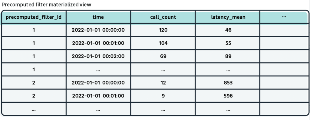
Step 4:
The reading componentcan convert a complex query to precomputed_filter.id = xxx and query the MV to return metrics of calls matching the complex query.
Example Pseuode Query:
SELECT SUM(call_count)
FROM precomputed_filter_view
WHERE time > toDateTime(‘2022-06-01 00:00:00’)
AND time < toDateTime(‘2022-06-01 12:00:00’)
AND precomputed_filter_id = ‘1’
How Do We Do Grouping?
precomputed_filter.id = xxx only handles the filtering part, if the query asks for metrics grouped with a tag like endpoint.name , we need to handle this with additional steps.
During the process, if a call matches the filter, we need to subtract the value of the grouping tag endpoint.name from the call and also store this tag in an additional column. The column will also be included in the MV placed after the precomputed_filter_id and time columns in the sort key.
Example Pseuode Query:
SELECT precomputed_filter_group, SUM(call_count)
FROM precomputed_filter_view
WHERE time > toDateTime(‘2022-06-01 00:00:00’)
AND time < toDateTime(‘2022-06-01 12:00:00’)
AND precomputed_filter_id = ‘1’
GROUP BY precomputed_filter_group
Conclusion
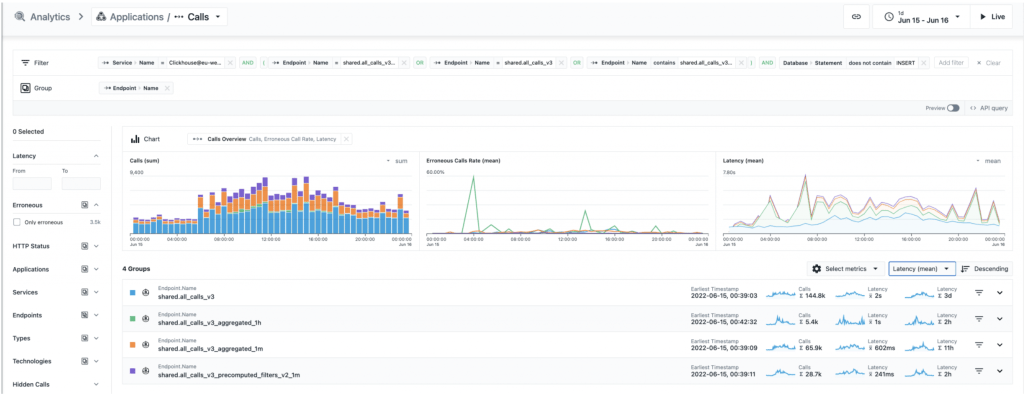
This image shows a very detailed analysis of the queries made by Instana customers in the Europe region over the course of a day, broken down by different tables and views. With the pre-calculated filter, we can see that the queries are almost 10x faster than the original searches table and 3x faster than a query optimized for the same bucket size (1min).
Limitations and Future Improvements
The biggest limit is that a query can only be optimized after it is first saved as a precomputed filter. It works well for recurring queries that users make regularly. However, if a user runs an ad-hoc query in unbounded analytics for the first time in the past day, the optimization won’t kick in right away. To limit the load on the pipeline, we also disable a precalculated filter after a period of inactivity.
Some complex queries can be predicted if configured in a custom dashboard or alarm. In these cases, we can use the configuration to create precomputed filters; so users can quickly see metrics and charts even if they open the custom dashboard or jump from an alert to unbounded analytics for the first time.
Share this blog post on social media!
Contact us to get detailed information about instana!